

Neural Networks come in many flavors and varieties. Convolutional Neural Networks (ConvNets or CNN) are one of the most well known and important types of Neural Networks. They are mainly used in the context of Computer Vision tasks like smart tagging of your pictures, turning your old black and white family photos into colored images or powering vision in self-driving cars. Recently researchers have also started exploring them in the domain of Natural Language Processing. One other noteworthy application of CNN is drug discovery — they allow to predict interactions between molecules and biological proteins, which paves the way for discovering new groundbreaking medical treatments. Fascinating, isn’t it?! So let’s try to understand the building blocks of these “seeing” neural networks.
(Before proceeding, I am assuming that you have a clear understanding of the basics of Neural Networks. If not, please read this post first.)
How do we teach computers to “see”?
Our brains have the capacity to process visual information within as little as 13 milliseconds. To put this into perspective, it takes us 300-400 ms to blink our eyes! And all of this happens without us even realizing the complex mechanism going on in our brains. However, if we want machines to understand visual information, we need to understand how to represent images in a machine readable format.
Image Representation
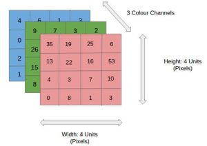
Neural Networks can only work with numbers. To a computer an image is nothing but a grid of numbers or pixel values that represent how dark each pixel is:
A colored image is said to have three channels – red, green and blue. Each channel is represented as a grid (or matrix) of pixel values ranging from 0 to 255. So our machine representation of a standard image from a digital camera would be three matrices stacked on top of each other, where the size of these matrices would be given by the height and width of the image. Please note that a gray-scale image would only have one channel, i.e., it would be a single matrix with pixel values ranging from 0 to 255, with 0 indicating black and 255 indicating white (like in the above representation of the digit 8).
Architecture of CNN
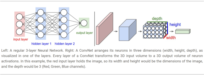
CNN are similar to classical fully-connected neural networks — they’re made up of layers of neurons and work with weights and biases. (“Fully-connected” means that every node in the first layer is connected to every node in the second layer). Each neuron receives some numbers as inputs, does a linear mapping and optionally applies a nonlinear activation function to its output.
What makes convnets special and suitable for working with image data is that CNN can deal with inputs in 3D format (width, height and depth), instead of just linear arrays like in classical neural networks. Each layer takes as input a 3D volume of numbers and outputs a 3D volume of numbers. CNN are able to do this because they possess two special layers: Convolution layer and Pooling layer.
The figure below shows the main architectural difference between a traditional and a convolutional neural network.
The main components of a CNN architecture are:
- Convolution layer (with some non-linearity like ReLU)
- Pooling layer
- Fully Connected Layer (the final output layer)
Let’s break-down each of these layers and try to understand what happens to our input pixels as they move through the network.
Convolution layer
When we see a cat, we are able to recognize it independently of where the cat is sitting or whatever else is going on in the rest of the image. For us, the identity of an object is not tied to its position in the image a.k.a. translation invariance. To make Neural Networks understand images, we need to be able to pass this type of “common sense” to them as well. This is where a process called Convolution comes in.
Convolution allows us to extract features from our input image. In simple words, we slice our input image into small tiles, apply a special transformation on each of these small tiles and save the output as a new (smaller) representation of our original tile. As a result, each of the smaller output ends up with the most interesting parts of the original larger tile, i.e., features of the input image get extracted.
The “smaller tiles” are obtained by using a filter matrix that we slide over our original matrix of pixel values to compute the convolution operation. Let’s say that we have a 5 x 5 image, whose pixel values are only 0 and 1, and a 3 x 3 filter matrix. Then, the Convolution of the 5 x 5 image and the 3 x 3 matrix can be computed as shown in the animation below:
What is happening in this animation? We slide the orange filter matrix over our original image (green matrix). For every region of overlap, we compute element by element multiplication or dot product between the two matrices and save the output (a single number) into the pink matrix. After each matrix multiplication step, the orange filter slides forward by one pixel at a time, also known as stride. The pink output matrix is also known as the Feature Map or Activation Map because the filter acts as a feature detector for our input image.
Changing the values of the filter matrix allows us to detect different features and hence obtain a different Feature Map. For example, if we are interested in detecting edges in an image, our filter will be different than the one used for detecting curves.
Here is a visual example showing one such transformation:
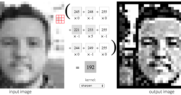
The 3 x 3 filter applied to sharpen the face is also shown separately below for clarity. (Sharpen operation emphasizes differences in adjacent pixel values) The output, 192, is obtained by multiplying the pixel values in the red tile (top-right of the left image) with this sharpen-filter.

You can checkout the source of the above face-image to play with such transformations. You’ll be able to see how two different filters generate two different feature maps from the same original image.
- Please note that the values of these CNN-filters are learnt during training. But the number of filters is specified as input parameter to a CNN (hyperparameters). A high number of filters means that the CNN would be able to extract more features and hence you get a model better equipped to work with new unseen inputs. The number of filters used is also called Depth. Also note that the number of parameters to be learnt (weights and biases for the filters) stays small even if the size of the input image is increased.
- If we increase the stride size — we shift the filter forward by more than one pixel at each step — the output matrix or Feature Map will be smaller and there will also be fewer overall applications of the filter.
Did you notice something missing in the animation with the green and orange matrices? How can we apply the filter to the first or last elements of a matrix, as they don’t have any neighboring elements to the top and left or bottom and right respectively? To not miss information at the edges, it is common to add zeros at the borders of the input matrix, zero-padding — all elements falling outside the original matrix are assigned to be zeros. In this way the sliding and filtering operation can cover all the pixels, including the ones at the borders.
Earlier I had mentioned that CNN allow us to preserve translation invariance. Now we can see that the filter stays the same as we vary spatial position (slide it across the input image). Once the neural network has learnt to get “excited” about a certain feature like an edge, it has learnt to spot that edge at any spatial position — spatial translation of features around the image doesn’t matter anymore.
After the Convolution operation, a non-linear activation function (ReLU) is applied to the results. And as we had discussed in the previous post, the activation function allows us to introduce non-linearity, because up till now, all we had done was to perform some multiplication between matrices — linear operations. The non-linear or ReLU layer sets all negative values in the Feature Map to zero. The resulting output matrix is called a Rectified Feature Map.
Pooling Layer
This is an easy to understand layer. Here we simply perform downsampling, i.e., reduce the size of the Feature Map. The output is called a Pooled Feature Map. Pooling allows to reduce computational cost, avoid overfitting and to have a fixed sized output (regardless of the size of the filters or the size of the input image).
The most common form of pooling is called Max Pooling:
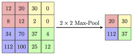
As you can notice in the image above, in Max Pooling we define a window of a given size, e.g., 2 x 2, and then simply pick the largest element from the feature map within that window. The largest number becomes the representative of the features present in its window, and we do not care about the position where the max appeared — this also provides basic positional invariance. Max Pooling is the most commonly used approach. However, instead of taking the largest element from the window, it is also possible to take the average or sum of all the elements. In the latter case, the pooling operations are called Average Pooling or Sum Pooling.
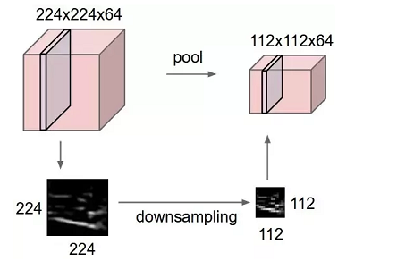
Pooling is done independently on each depth of the 3D input, so after the pooling operation the image depth remains the same.
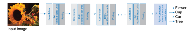
Let’s summarize what we have seen so far: we have Convolution, ReLU & Pooling layers. Convolution layers produce N feature maps based on N filters. ReLU is applied to add non-linearity to the output of the convolution operation, and the resulting rectified output is passed as input to the Pooling layer, which in turn reduces the spatial size of the Feature Map while preserving its depth. We can have series of these layers as depicted in the image below. And they all work together with the aim of extracting useful features from the input image.
Fully Connected Layer
At the end of a CNN, the output of the last Pooling Layer acts as input to the so called Fully Connected Layer. There can be one or more of these layers (“fully connected” means that every node in the first layer is connected to every node in the second layer).
Fully Connected layers perform classification based on the features extracted by the previous layers. Typically, this layer is a traditional ANN containing a softmax activation function, which outputs a probability (a number ranging from 0-1) for each of the classification labels the model is trying to predict.
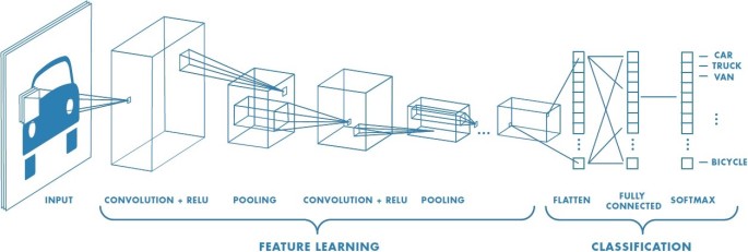
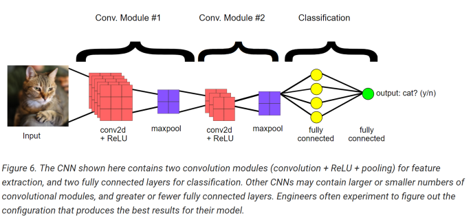
The figure below shows the end-to-end structure of a simple CNN.
The Overall Training Process
- Initialize all filters values, parameters and weights with random values.
- Apply Convolution modules followed by the Fully-Connected Layer(s) and obtain final class probabilities.
- Calculate the total output error. (At first this will be high because we started with random values)
- Use backpropagation and gradient descent to update filter values and weights so that the output error is minimized. Note that the parameters like filter size and number of filters do not get updated – they are to be specified at the beginning of the training process.
- Steps 2-4 are continued in a loop until the output error reaches the desired value.

As shown in the image above, the first hidden layers get activated or “excited by” simple shapes or features like curves and edges. As we progress through the hidden layers, the neurons start looking at more and more complex shapes and at a wider input field, until eventually they are able to understand a complete representation of the input pixels — they build edges from pixels, shapes from edges, and more complex objects from shapes.
State-of-the-art CNN architectures
I have described the basic building blocks of any CNN. There is more to the picture: the deep learning research community is actively investing in groundbreaking work to improve upon the existing CNN architectures. The ImageNet project is a large visual database designed for use in visual object recognition research. Since 2010, it runs an annual software contest, the ImageNet Large Scale Visual Recognition Challenge (ILSVRC) and the winner gets the “state-of-the-art” title (Computer Vision Olympics!)
VGGNet is one example of a winning architecture (2014 winner) . It improved on the previous CNN by showing that the number of layers are critical for performance. You can read more about their 16-19 layers models here. ResNet, AlexNet, GoogLeNet and DenseNet are some other such winners. These networks pre-trained on the Image-Net dataset can be retrieved and reused in Keras (or other deep learning frameworks) in a very trivial way.
End Notes
CNN are inspired by the human brain. Some researchers in the mid 90s studied the brains of cats and monkeys to analyze how a mammal’s brain perceives visual stimuli. They showed that there are two types of cells: Simple cells which are able to identify basic shapes like lines and edges and complex cells which respond to larger receptive fields and their outputs are independent of spatial positioning. This research was at the basis of the work that went into creating computers that could “see” – the first CNN, LeNet5.
I hope you found this post helpful and that now you have an intuitive understanding of Convolutional Neural Networks. If you are interested in going deeper, you can refer to this material by Stanford. Also, stay tuned for a hands-on tutorial. In the meanwhile, Happy Learning!
. . .
If you enjoyed reading this post and you want to continue on this ML journey, press the follow button to receive the latest right at your inbox!
References and Further Reading
- CS231n Convolutional Neural Networks for Visual Recognition
- Feature-Visualization
- Image Kernels
- Convolutional Neural Networks
