Deep Learning Series, P3: Understanding Recurrent Neural Networks

1. Why RNNs?

Your smartphone predicting your next word when you are typing, Alexa understanding what you are saying or tasks like making stock market predictions, understanding movie plots, composing music, language translation and human learning: can you tell what is the common theme in this list? These are examples where sequence of information is crucial.

For example, look at the following sentence:

I like to have a cup of ___ for breakfast.

You are likely to guess that the missing word is coffee. But why didn’t you think of sandwich or ball? Our brains automatically use context, or words earlier in the sentence, to infer the missing word. We are wired to work with sequences of information, and this allows us to learn from experiences — “we are but a total of our experiences”. From language to audio to video, we are surrounded by data where the information at any point in time is dependent on the information at previous steps. This means that for working with such data we need our neural networks to access and understand past data. Vanilla neural networks cannot do this because they assume that all inputs and outputs are independent of each other; there is a fixed-sized vector as input and a fixed-sized vector as output. And this is why Recurrent Neural Networks come into play.

Note: Before proceeding, I am assuming that you have a clear understanding of the basics of Neural Networks for going through this article. If not, please read this post first.

Also, if you are not interested in learning about the mathy details coming in the next section, you can scroll down to a fun demo application in Section 4!

2. What are RNNs?

RNNs are called “recurrent” neural networks because they can work with sequences by having a mechanism that can persist and access data from previous points in time. This allows the output to be based on time dependent or sequential information (you can try to think of a memory based system). RNNs operate over sequences of vectors as shown in the diagram below.

Each rectangle is a vector and arrows represent functions (e.g. matrix multiply). Input vectors are in red, output vectors are in blue and green vectors hold the RNN’s state. From left to right: **(1)** Vanilla mode of processing without RNN, from fixed-sized input to fixed-sized output (e.g. image classification). **(2)** Sequence output (e.g. image captioning takes an image and outputs a sentence of words). **(3)** Sequence input (e.g. sentiment analysis where a given sentence is classified as expressing positive or negative sentiment). **(4)** Sequence input and sequence output (e.g. Machine Translation: an RNN reads a sentence in English and then outputs a sentence in French). **(5)** Synced sequence input and output (e.g. video classification where we wish to label each frame of the video).

Let’s try to intuitively understand the inner workings of RNNs by looking at how we could enhance a vanilla neural network to remember past data.

Say that we have 3 inputs X0, X1, X2. In a traditional neural network, our ouputs would be given by applying a non linear function, f, to the dot product of the weight matrix W and the input X (summed with a bias, b):

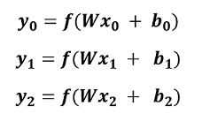
In the figure above, you can see that each output is only dependent on its current input and there is no correlation with any of the previous inputs. How could we alter the equations above to capture past information? Let’s try using the output of the previous hidden layer and the input X at the current point in time as inputs for the new hidden layer:

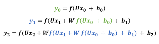
We just managed to introduce the concept of learning from past experiences in our network — at each point in time we are looking at the previous computations as well. Basically, the above equations translate to the following property of RNNs: these networks have loops for persisting and accessing information from sequences as input.

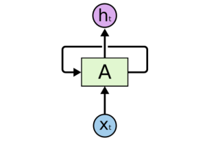
: Recurrent Neural Networks have loops.

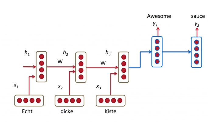
Let’s view the unrolled version of a RNN for a clearer understanding:

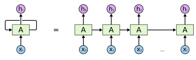
As you can see in the image above, the RNN first takes x0 from the input sequence and it outputs h0. Then h0, along with the next element in the sequence x1, becomes the input for the next step. Similarly, h1 from the second step becomes the input, along with x2, for the next timestep and so on.

We have just learnt how to allow RNNs to have context from previous information. Now let’s put all of this together in the form of complete equations (if you are feeling a bit lost, take a look again at the equations we had derived earlier — we are just rewriting them in a more compact manner):

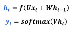
As you can see, the hidden state ht acts as the memory of the network because it captures information about what happened in all the previous timesteps.

The weight matrix U allows the hidden layer to extract information from the current input. And the weight matrix W is what distinguishes RNNs from a typical neural network — the dot product of W with information propagated from the previous hidden layers allows RNNs to work with sequences. f could be any activation function, e.g., ReLU. The softmax function allows us to obtain class probabilities as outputs. Also, you could have an additional bias term b in the equations above (omitted for simplicity).

Note that unlike a traditional deep neural network which uses different parameters at each layer, RNNs share the same parameters ( $U, V, W$ above) across all timesteps because they are performing the same task at each step, just with different inputs. This greatly reduces the total number of parameters to learn.

3. RNNs extensions: LSTMs

RNNs are one of the best deep NLP model families. However, there is one problem. They cannot look more than n timesteps back. They suffer from a problem known as the vanishing gradient problem: as the depth of the network increases, the gradients flowing back in the back propagation step become smaller and smaller. As a result, the learning rate becomes very slow and the hidden state cannot capture long term dependencies. In other words, RNNs remember things for just small durations of time, so if we need some particular information after a short time, it may be retrievable, but once a lot of sentences are fed in, this information gets lost along the way.

For instance, let’s say that we want to predict the last word in the following text:

“I grew up in Italy. I moved to Norway a month ago. I speak fluent Italian.”

Recent information, “I speak”, suggests that we are trying to predict the name of a language. But to decide which language, we need the context of “Italy”, from further back. As the gap between the available information and the place where it’s needed grows, RNNs are not able to form a connection. Here an extended version of RNNs called LSTMs comes to rescue. LSTMs are very similar to RNNs in terms of architecture. The main differnce is that LSTMs have a more powerful equation for computing the hidden state.

When new information is added, RNNs transform the existing information completely by applying the function f. This means that the information is modified as a whole, without any notion of “important” vs “not so imporant” information. On the other hand, LSTMs make small modifications to the information by multiplications and addition so that they can selectively remember or forget things.

LSTMs have cells which act as their memory. These cells have a mechanism for deciding what to keep and what to discard from memory. They are essentially like black boxes which take as input the previous state $h_{t-1}$ and current input $x_t$ . Once they have done their “memory clean-up”, they combine the previous state, the current memory and the current input. This allows LSTMs to capture long term dependencies. I’ll go into the details of LSTMs in a separate post. In the meanwhile, you can read more about them here.

4. Example applications of RNNs

First, some fun and creative ways of using RNNs!:D

Sketch-RNN — Draw together with a Neural Network

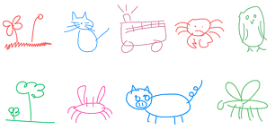
Sketch RNN is an experiment that lets you draw together with a RNN model. The neural net was taught to draw by Google by training it on millions of doodles collected from the Quick, Draw! game. Once you start doodling an object, Sketch-RNN comes up with many possible ways to continue drawing this object based on where you left off. The model can also mimic your drawings and proce similar doodles. This is a great example of how we can use machine learning in fun and creative ways.

You can try it out here.

And here are some other suggestions of fun applications for you to play with: RNN generated political speeches, Harry Potter written by AI and Shakespeare style poems generated by neural networks.

Now, let’s look at some common (real-world) applications:

Machine Translation

In the last few years, RNNs have been successfully applied to a variety of problems: speech recognition, language modeling, language translation and image captioning —they are most widely used for Natural Language Processing tasks.

One famous application of RNNs is Machine Translation. Machine Translation is most commonly done via end-to-end neural networks where the source sentence is encoded by a RNN called Encoder and the target words are predicted using another RNN called Decoder. The Encoder reads a source sentence one symbol at a time and then summarizes the entire source sentence in its last hidden state. The Decoder uses back-propagation to learn this summary and returns the translated sentence.

As you can observe in the image above, the first output is only emitted after having seen the entire input sequence because the first word in one language can be dependent on the last word of the sentence in another language.

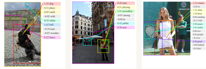
Generating captions for images

Coupled with Convolutional Neural Networks, RNNs have been used in models that can generate textual descriptions for unlabeled images (e.g., you can think of YouTube’s closed captions).

*Source: http://cs.stanford.edu/people/karpathy/deepimagesent/*

End Notes

I hope that you found this article helpful in gaining an intuitive understanding of the core of RNNs. The range of applications and the power they give us is amazing. For example, we are just at the beginning of AI driven conversations. I am excited to see what the future has in store for us in regards. What about you?

. . .

If you enjoyed reading this post and you want to continue on this ML journey, press the follow button to receive the latest right at your inbox!

References and Further Reading

Source